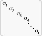
 where D is a diagonal matrix containing the singular values. D, as one might guess, looks like this:
 where
where  are the singular values of the matrix A with rank r. A full rank decomposition of A is usually denoted like this:
  .
.On the previous page, we learned that singular value decomposition breaks any matrix A down so that A = U*S*V'. Let's take a closer look at the matrix S.
Remember S is a matrix of the form  where D is a diagonal matrix containing the singular values. D, as one might guess, looks like this:
 where
where  are the singular values of the matrix A with rank r. A full rank decomposition of A is usually denoted like this:
  .
.
We can find a reduced rank approximation (or truncated SVD) to A by setting all but the first k largest singular values equal to zero and using only the first k columns of U and V.
Why are we using this particular decomposition for our rank k approximations? According to the optimality property, singular value decomposition gives the closest rank k approximation of a matrix. What do I mean by close?
A theorem proven by Eckart and Young shows that the error in approximating a matrix A by Ak can be written:
So what k should we choose? If we choose a higher k, we get a closer approximation to A. On the other hand, choosing a smaller k will save us more work. Basically, we must choose between time and accuracy. Which do you think is more important? How can we find a good balance between sacrificing time and sacrificing data?
Activity 4 One trick is to look at and compare all the singular values of your matrix. Create a random matrix A in MATLAB using the randintr command we used earlier. Now calculate only the singular values of your matrix with the command
svd(A).
Now plot these values by entering
plot(svd(A)).
Note how the singular values decrease. When we multiply U, S, and V back together, the larger singular values contribute more to the magnitude of A than the smaller ones. Are any of the singular values of your matrix A significantly larger than the others?
Now create the following matrix N in MATLAB:
Again calculate the singular values (rather than the whole decomposition) and plot the values. Are any of the singular values for this matrix significantly higher than the others? What do you think we should choose as our k for this matrix?
Download the following m-files for the following MATLAB activity.
cityplot.mDo you still have your term-by-employee matrix stored? If not, re-enter it into MATLAB and store it as matrix A (or another variable you prefer).
Drag the files into the current directory and enter the command
displaySVD2(A)
A window should pop-up showing two "city plot" graphs: one of the rank 1 approximation of your matrix and one of the matrix itself. The graphs should look something like this:
Look at each graph from different angles by clicking on the "rotate" icon at the top of the window, then clicking and dragging the graph around.
When you're done looking at these two graphs, hit the space bar and the rank 2 approximation will appear. Continue to examine and compare the graphs until you have seen all k approximations.
If you had to choose a k based on these graphs, which would you choose? Why? What do your co-workers think?
Hopefully this exercise gave you a better idea of what the rank k approximations look like as k gets closer and closer to r (or the rank of the original matrix).
SVD has been useful in many other fields outside of information retrieval. One example is in digital imaging. It turns out that when computers store images, they store them as giant matrices! Each numerical entry of a matrix represents a color...sort of like a giant paint-by-number. How could SVD be useful here?
Activity 6
Make sure the ATLAST commands are in your current directory again, then enter the commands:
 load gatlin2

image(X), colormap(map)
This will create a 176x260 matrix X representing the image you see after entering the second command.
Now enter ATLAST command svdimage(X,1,map)and a new window containing two images should appear. The one on the left is the original image, and the one on the right is a rank 1 approximation of that image. Hit any key and the rank increases by one.
What would be a good k for your image? How much storage space would the computer save by storing this approximation in decomposed form (mxn numbers to store for the original matrix vs. mxk + k + nxk numbers to store for the decomposed rank k approximation)?
For completely dense matrices, like images, we can obviously save a lot on storage. Would we save a lot on storage for a sparser matrix like our term-by-document matrices?
Computers store sparse matrices in a different way; they only store the non-zero entries of the matrix. Storage savings is probably not going to be our motivation for using rank-k approximations. So why do we use it?
As you may recall, the equation for calculating the cosine of the angle between a query vector and another vector is:
Since Akej equals the jth column of the rank k matrix A, then we can rewrite the formula:
 then we can simplify the formula to:
 Berry & Brown, 1999. This is still a bit of an expensive calculation, but not nearly as expensive as processing a query without SVD.
Not many search engines are still using the vector space model and SVD to process queries. Is Company Enterprises the only company still taking advantage of this method? Not completely. Some companies are still using Latent Semantic Indexing (LSI) which is a method that uses SVD. According to Langville, 2005,
		the LSI method manipulates the matrix to eradicate
		dependencies and thus consider only the independent,
		smaller part of this large term-by-document matrix.
		In particular, the mathematical tool used to achieve the
		reduction is the truncated singular value decomposition
		(SVD) of the matrix.
Here's an example of how a company is using LSI to its advantage.
Congratulations! You have now learned all you need to know about the vector space model and singular value decomposition and so have completed your training for Company Enterprises. Continue on to the next page for your first assignment as an official employee of Company Enterprises.
Or Jump to a page!letter 1 2 3 4 5 6
This material is based upon work supported by the National Science Foundation under Grant No. 0546622. Any opinions, findings, and conclusions or recommendations expressed in this material are those of the author(s) and do not necessarily reflect the views of the National Science Foundation.